Bulk water#

Measuring the NMR relaxation time of water

MD system#

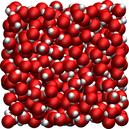
Water molecules simulated with lammps - NMR relaxation time calculation

The system is a bulk liquid water with a number $N$ of water molecules, where $N$ was varied from 25 to 4000. The simulation box was cubic, with equilibrium dimensions ranging from $(0.9\,\text{nm})^3$ to $(4.9\,\text{nm})^3$. The trajectory was recorded during a $8\,\text{ns}$ production run performed with the open source codes LAMMPS (for the smallest systems) and GROMACS (for the largest systems). Simulations were performed in the NPT ensemble using a timestep of $2\,\text{fs}$. The imposed was temperature $T = 300\,^\circ\text{K}$, and the pressure $p = 1\,\text{atm}$. The positions of the atoms were recorded in the prod.xtc file every $\Delta t$, with $\Delta t$ ranging from $0.2\,\text{ps}$ to $32\,\text{ps}$.

Results#

Both intra and inter-molecular correlation functions were extracted, and the respective intra and inter NMR spectra were calculated. The total NMR spectrum $R_1$ was also calculated.

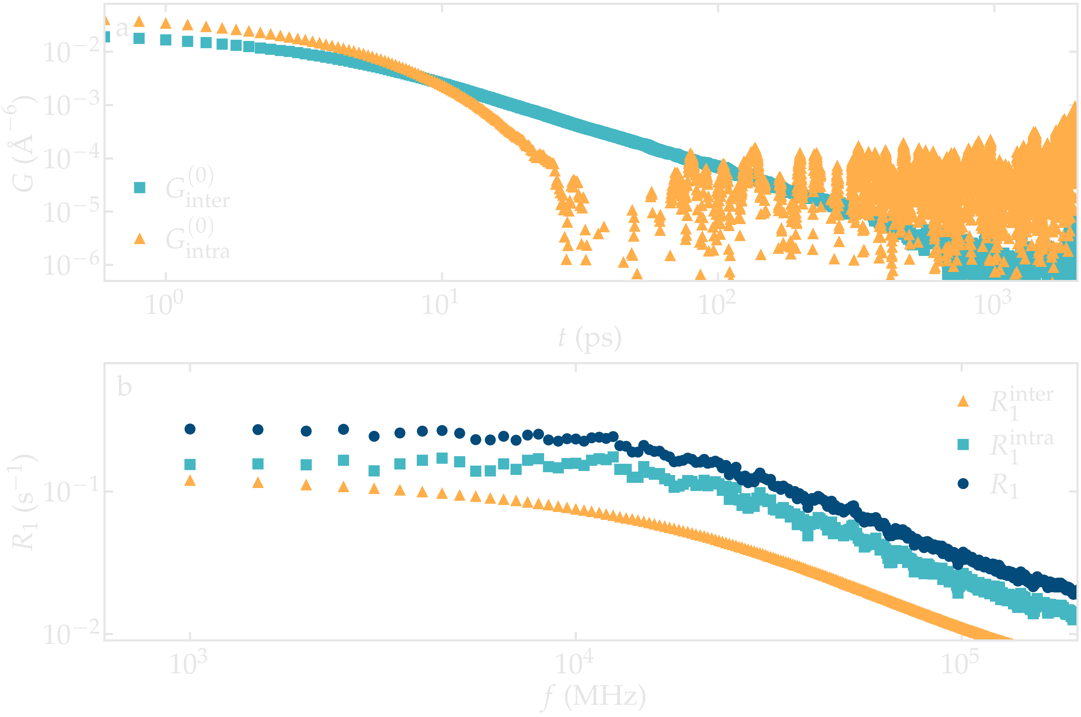
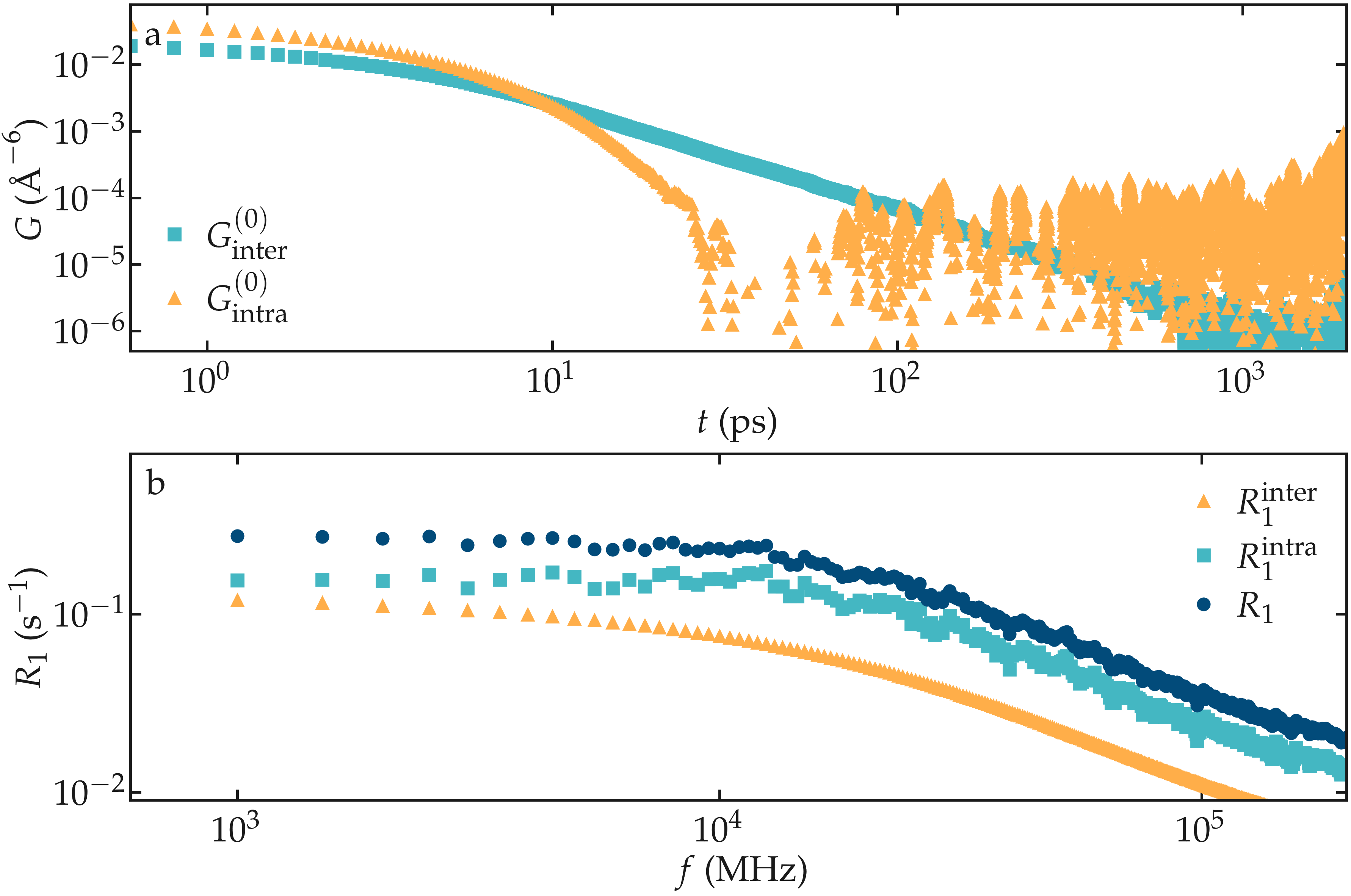
Figure: a) Correlation function $G^{(0)}$ as extracted from the bulk water simulation with $N = 4000$ and $N = \Delta t = 1\,\text{ps}$. b) Corresponding NMR spectra $R_1$.

The inter-molecular correlation function shows the expected power law at longer time, while the intra-molecular correlation decreases faster with time.

Our results also show that the relaxation is dominated by intra-molecular contribution, as expected for water under ambient conditions [2]. For the lowest frequency considered here, the spectrum $R_1$ is almost flat.

Let us first visualize how $r_{ij}$ and $\Omega_{ij}$ evolve with time in the case of a bulk water simulation at 300 K. For such bulk systems, it is known that the correlations functions are proportional to each others [3], so only $G^{0}$ and $J^{0}$ will be evaluated, which depends only in the polar angle $\theta_{ij}$ as $Y^{0}_2$ is independent from the azimuthal angle $\varphi$.

First, let us have a look at the intramolecular motion within a single water molecule. As expected for the rigid water model used here (TIP4P/$\epsilon$), the average distance $r_{ij}$ between the two hydrogen atoms of the same molecule remains constant (within the uncertainty of the shake algorithm used to maintain the water molecule rigid), while the polar angle $\theta_{ij}$ fluctuates with time, following the rotation of the water molecule (see the Figure below). The fluctuations of $\theta_{ij}$ with time lead to fluctuations of the function $F_{0}^{(2)}$ (see Eq. (4)) between a higher bound given by $(3 \cos^2 0 - 1 ) / a^3 \approx 0.58\,A^{-3}$, where $a \approx 1.51\,A$ is the typical distance between the two hydrogen atoms of the water molecule, and a lower bound $(3 \cos^2 \pi/2 - 1 ) / a^3 \approx -0.29\,\,A^{-3}$.

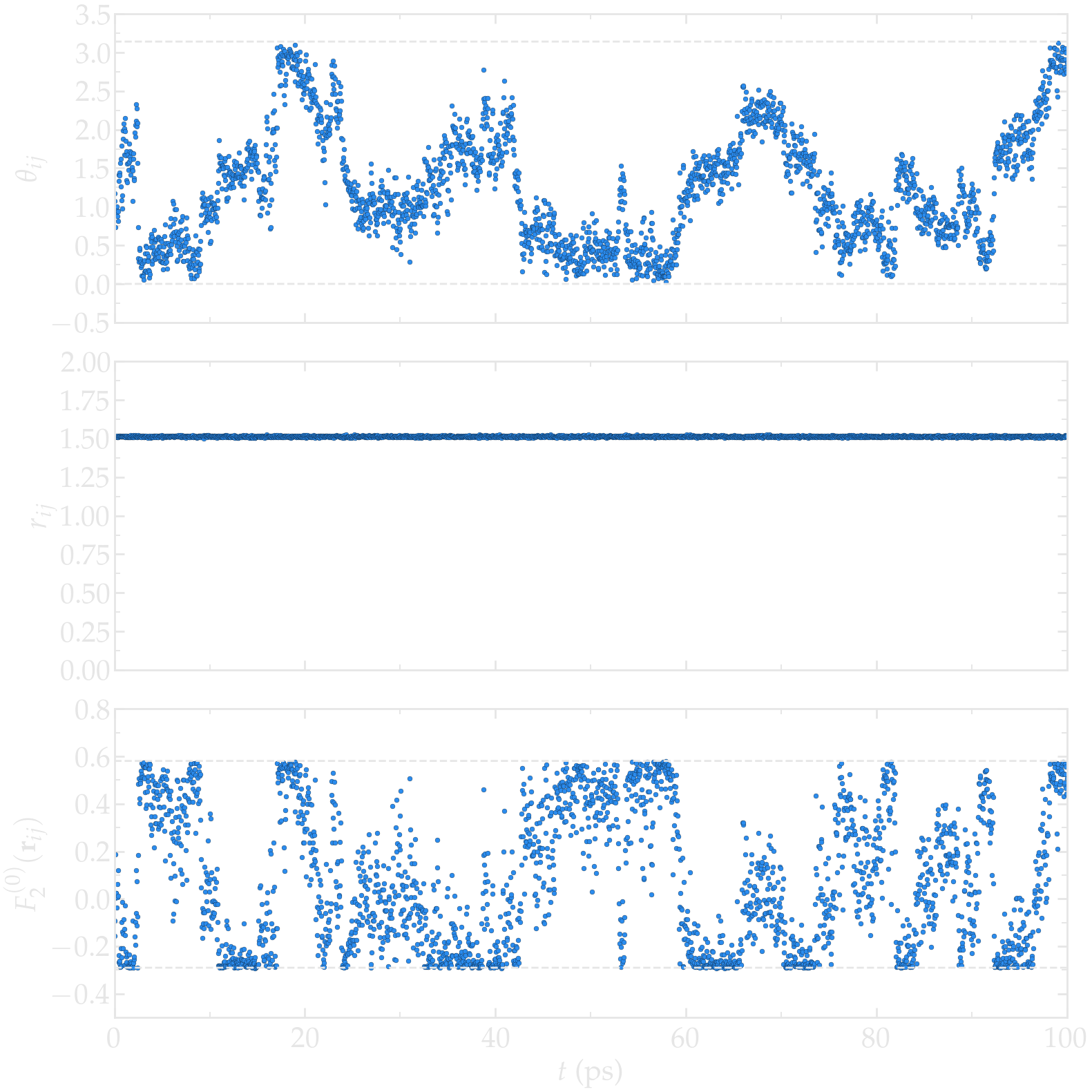
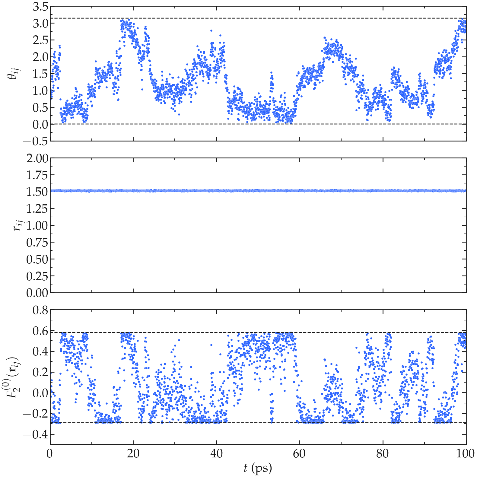
Figure: a) $\theta_{ij}$ as a function of the time $t$, where $i$ and $j$ refer to two hydrogen atoms located within the same water molecule. a) $r_{ij}$ as a function of time. c) $F_{2}^{(0)}$ as a function of time. The temperature is 300 K, and the total number of water molecules is 3000.

Second, let us have a look at the intermolecular motion between two hydrogen atoms from two different molecules. In that case, $r_{ij}$ fluctuates significantly between $\approx 2.5 A$, corresponding to the shortest typical distance between two molecules that are next to one another, to larger values (potentially as large as the box permits). As can be seen, the function $F_{0}^{(2)}$ reaches its largest absolute values when $r_{ij}$ is the shorter.

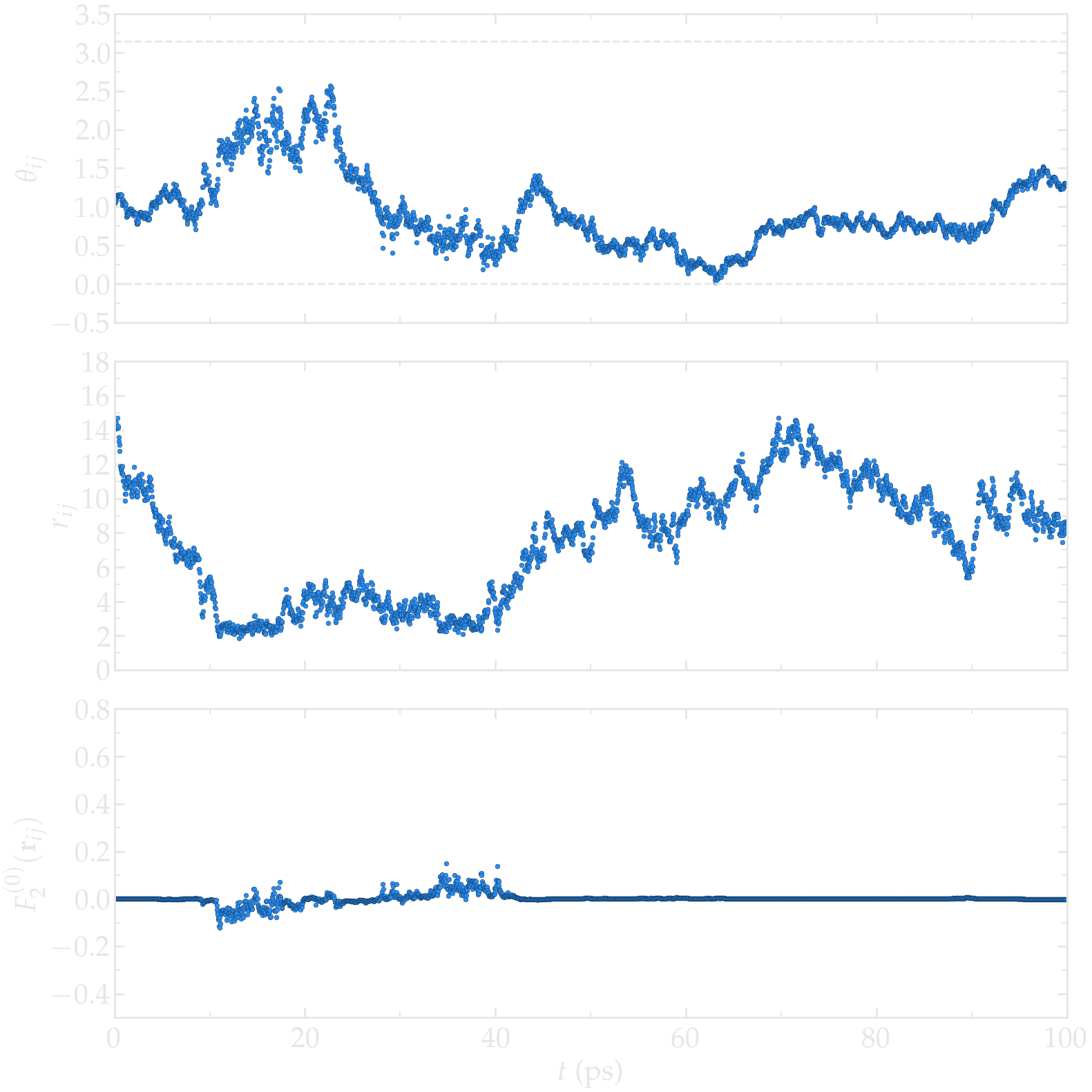
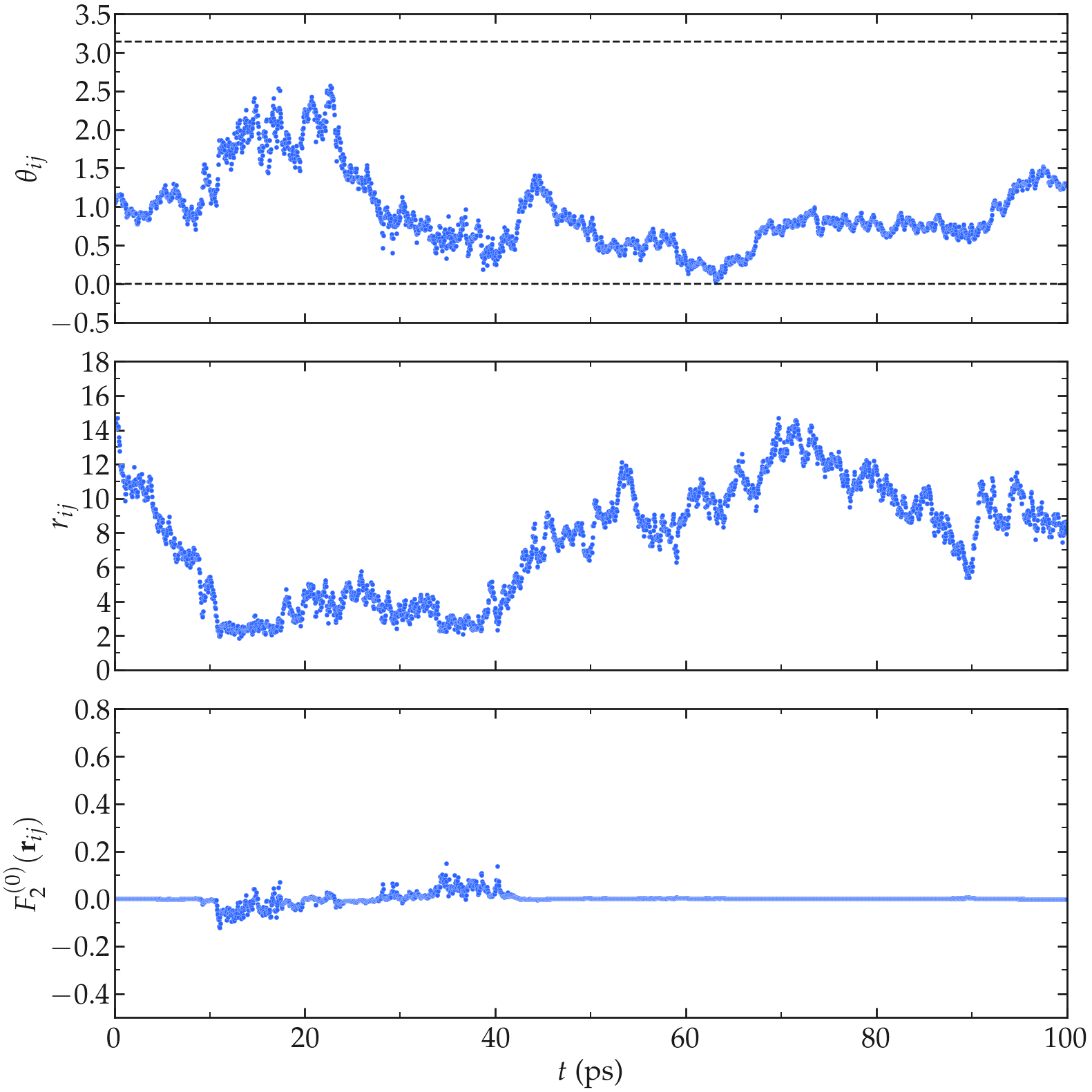
Figure: a) $\theta_{ij}$ as a function of the time $t$, where $i$ and $j$ refer to two hydrogen atoms located within two different water molecules. a) $r_{ij}$ as a function of time. c) $F_{2}^{(0)}$ as a function of time. The temperature is 300 K, and the total number of water molecules is 3000.

From the fluctuating quantities $F_{0}^{(2)}$ summed up over all the available pair of spins, one can extract the two correlation functions $G_\textrm{intra}^{(0)}$ and $G_\textrm{inter}^{(0)}$ (see Eqs. (2) and (3)). For comparison, the results obtained with two different temperatures 275 and 300 K are reported.

At short time $t < 40$ ps, the intra-molecular correlation functions follow and a decreasing exponential,

(1)#\[G_\text{intra} (t) = G_\text{intra} (0) \exp{(-t / \tau_\text{intra})},\]

where $\tau_\text{intra} = 6.3$ ps was used for $T = 300$ K and $\tau_\text{intra} = 3.2$ ps was used for $T = 275$ K, see the figure below. Exponentially decreasing correlation functions such as Eq. (1) are commonly used to describe systems for which the rotational diffusion is isotropic [4].

The inter-molecular correlation functions, however, scale as an exponential [i.e. Eq. (1)] only for time shorter than a few tens of pico-second, and show a clear scaling as $G_\text{inter} (t) \sim t^{-3/2}$ for large time which is a characteristic signature of the diffusion process controlling the motion of the molecules. The scaling $G_\text{inter} (t) \sim t^{-3/2}$ has long been predicted, and analytical expressions have been proposed by Ayant et al. [5] and Hwang and Freed [6], in the context of freely diffusing hard spheres. Following Ref [1], this expression is here referred to as a ADHF.

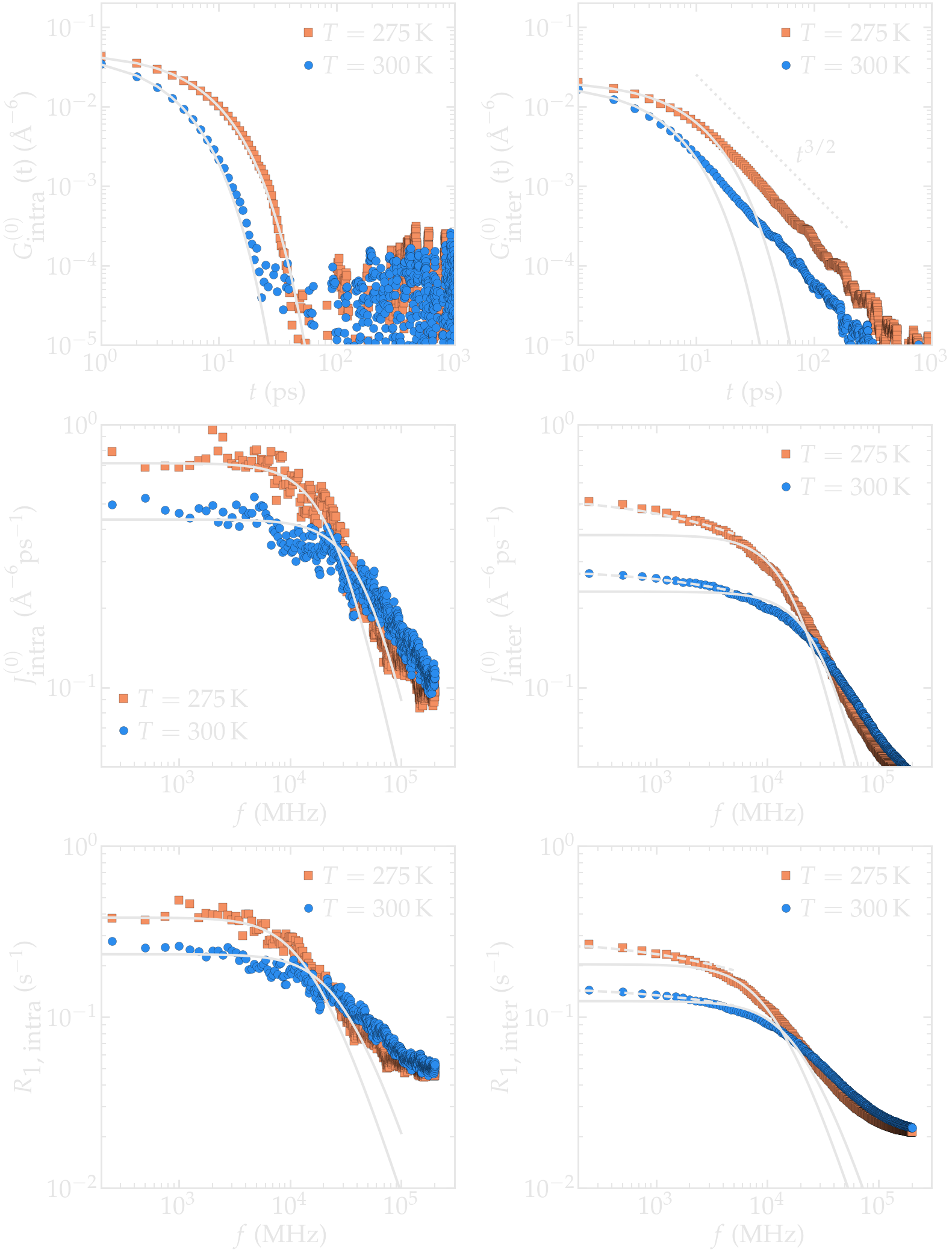
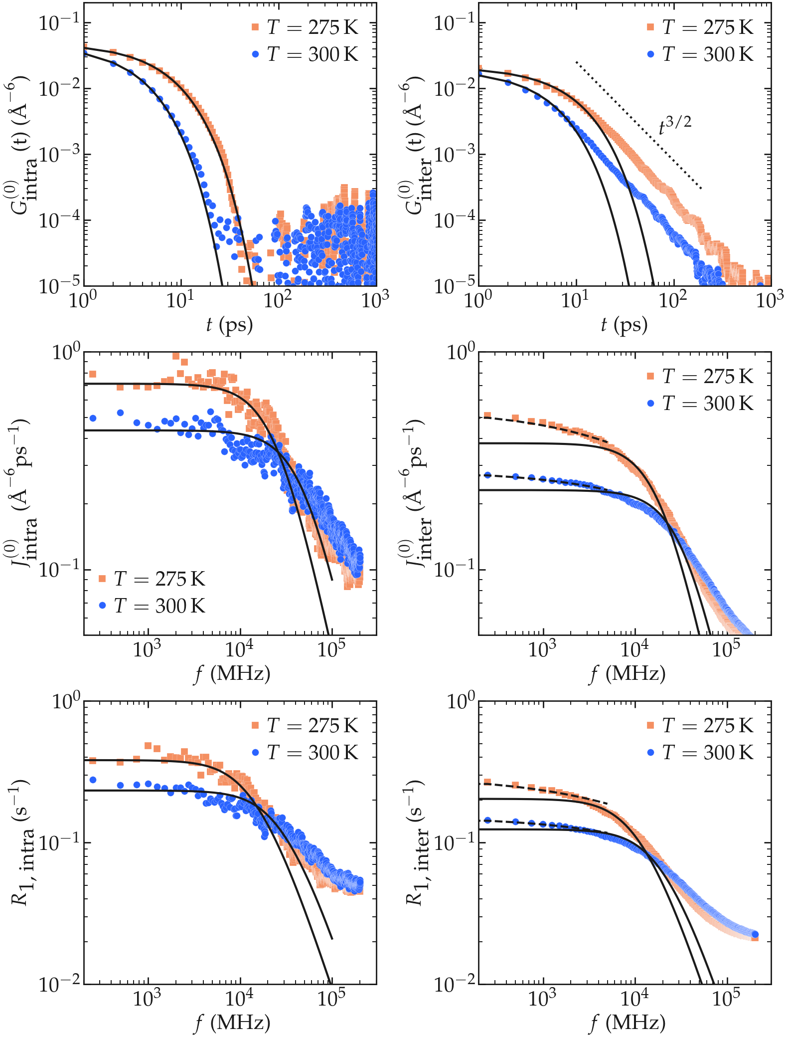
The intra molecular spectrum $J_\textrm{intra}^{(0)}$ can be reasonably well adjusted by a Lorentzian

(2)#\[J_\text{intra} (f) = G_\text{intra} (0) \dfrac{2 \tau_\text{c}}{1 + 4 \pi^2 f^2 \tau_\text{c}^2}\]

using $\tau_\text{c} = 6.3$ ps and $G(0) = 56300$ A⁻⁶ ps⁻² for $T = 300$ K and $\tau_\text{c} = 3.2$ ps and $G(0) = 59500$ A⁻⁶ ps⁻² for $T = 275$ K.

The inter molecular spectrum $J_\textrm{inter}^{(0)}$, however, does not follow the Lorentzian plateau, particularly at the lowest frequencies, which is consistent with the correlation function $G_\textrm{inter}^{(0)}$ decaying with time as a power law. In that case, and following closely Ref. [7], an exact analytical expression for the surface spectrum $J_\textrm{surf} (f)$ can be obtained from the first return passage time of a molecule between successive adsorption and desorption at the surface of a sphere, in the limit of a large diffusing reservoir:

(3)#\[J_\text{inter} (f) \sim \left[ 1 + A + B \sqrt{ 2 \pi f} \right]^{-1}.\]

Still from Ref. [7], one can deduce that $A = k r / D$ and $B = r / \sqrt{D}$ where $r$ is here the radius of the water molecule, $D$ the diffusion coefficient, and $k$ a phenomenological rate constant with the units of m/s. The frequency scaling as predicted by equation (3) is in good agreement with molecular dynamics results at frequency lower than $10^4$ MHz.