Dipolar relaxation

The system of interest here is an ensemble of identical spins characterized by a gyromagnetic ratio \(\gamma_I\) and spin quantum number \(I\). For \(^{1} \text{H}\), the most abundant isotope of hydrogen, \(I = 1/2\) and \(\gamma_I = 26.752\) rad/T/s. For \(^{13} \text{C}\), a natural and stable isotope of carbon, \(I = 1/2\) and \(\gamma_I = 6.728\) rad/T/s [25].

One assumption behind the theory presented here is that the cross-correlation terms can be neglected, see Ref. [4].

When the spin-lattice relaxation is dominated by fluctuations of the magnetic dipole-dipole interaction, as is the case for protons in molecular systems, the rates \(R_1 (\omega)\) and \(R_2 (\omega)\) are related to the spectral densities \(J^{(m)}(\omega)\) of these fluctuations via the Bloembergen-Purcell-Pound (BPP) equations [26]:

(1)\[ \begin{align}\begin{aligned}R_1 (\omega) & = & K \left[ J^{(1)} (\omega) + J^{(2)} (2 \omega) \right],\\R_2 (\omega) & = & K \left[ J^{(0)} (0) + 10 J^{(1)} (\omega) + J^{(2)} (2 \omega) \right] / 4,\end{aligned}\end{align} \]

where

\[K = \dfrac{3}{2}\left(\dfrac{\mu_0}{4 \pi}\right)^2 \hbar^2 \gamma^4 I (I+1),\]

where \(\mu_0\) is the vacuum permeability, and \(\hbar\) the Planck constant (divided by \(2 \pi\)). The constant \(K\) has the units of \(\text{m}^6/\text{s}^2\). The spectral densities \(J^{(m)} (\omega)\) in Eq. (1) can be obtained as the Fourier transform of the autocorrelation functions \(G^{(m)}(\tau)\)

\[J^{(m)} (\omega) = \int_0^\infty G^{(m)} (\tau) \cos(\omega \tau) \mathrm d \tau.\]

The spectral densities are a measure of the distribution of the fluctuations of \(G^{(m)}(\tau)\) among different frequencies, so they provide information on the distribution of the power available for causing spin transitions among different frequencies. The autocorrelation functions \(G^{(m)}(\tau)\) read

\[G^{(m)} (\tau) = \left< F_2^{(m)} [\textbf{r}_{ij} (t)] F_2^{*(m)} [\textbf{r}_{ij} (0)] \right>\]

where \(F_2^{(m)}\) are some complex functions of the vector \(\textbf{r}_{ij}\) between the spin pairs, with norm \(r_{ij}\) and orientation \(\Omega_{ij}\) with respect to a reference applied magnetic field, assumed to be in the \(\textbf{e}_z\) direction. The functions \(F_2^{(m)}\) read

\[F_2^{(m)} [\textbf{r}_{ij} (t)] = \alpha_m \dfrac{Y_2^{(m)} [\Omega_{ij} (t)]}{r_{ij}^3 (t)}\]

where \(Y_2^{(m)}\) are normalized spherical harmonics and \(\alpha_0^2 = 16 \pi /5\), \(\alpha_1^2 = 8 \pi /15\), and \(\alpha_2^2 = 32 \pi / 15\). Therefore, one can write for the correlation functions:

\[G^{(m)} (\tau) = \dfrac{\alpha_m^2}{N} \sum_i \sum_{j \ne i} \dfrac{Y_2^{(m)} [\Omega_{ij} (0)]}{r_{ij}^3 (0)} \dfrac{Y_2^{*(m)} [\Omega_{ij} (\tau)]}{r_{ij}^3 (\tau)},\]

where \(N\) is the number of spins.

Intra/inter contributions

Intra-molecular and inter-molecular contributions to \(R_1\) and \(R_2\) can be extracted separately, by splitting the correlation functions as:

(2)\[G^{(m)}_\text{intra} (t) = \dfrac{\alpha_m^2}{N} \sum_i \sum_{j \in M_i} \dfrac{Y_2^{(m)} [\Omega_{ij} (0)]}{r_{ij}^3 (0)} \dfrac{Y_2^{*(m)} [\Omega_{ij} (\tau)]}{r_{ij}^3 (\tau)},\]

(3)\[G^{(m)}_\text{inter} (t) = \dfrac{\alpha_m^2}{N} \sum_i \sum_{j \notin M_i} \dfrac{Y_2^{(m)} [\Omega_{ij} (0)]}{r_{ij}^3 (0)} \dfrac{Y_2^{*(m)} [\Omega_{ij} (\tau)]}{r_{ij}^3 (\tau)},\]

where \(j \in M_i\) and \(j \notin M_i\) refer to summation on spin from the same molecule as \(i\), and from different molecules as \(i\), respectively.

Intra-molecular relaxation is usually attributed to the rotational motion of the molecules, and inter-molecular relaxation to their translational motion. This is only an assumption that simplify the interpretation of results, and can lead to error [3].

Isotropic system

For isotropic systems, the correlation functions are proportional to each others, and only \(G^{(0)} (t)\) needs to be calculated.

In that case, \(G^{(0)} = 6 G^{(1)}\), and \(G^{(0)} = 6 / 4 G^{(2)}\) [19], and the spectrums can be calculated as:

\[ \begin{align}\begin{aligned}R_1 &=& \frac{K}{6} \left[ J^{(0)} (\omega_0) + 4 J^{(0)} (2 \omega_0) \right],\\R_2 &=& \frac{K}{6} \left[ J^{(0)} (0) + \frac{5}{2} J^{(0)} (\omega_0) + J^{(0)} (2 \omega_0) \right],\end{aligned}\end{align} \]

which require less computational time and less memory to achieve, as only

(4)\[ \begin{align}\begin{aligned}F_2^{(0)} [\textbf{r}_{ij} (t)] & = & \alpha_m \dfrac{Y_2^{(0)} [\Omega_{ij} (t)]}{r_{ij}^3 (t)}\\& = & \dfrac{3 \cos^2 \theta_\text{ij} (t) - 1}{r_{ij}^3 (t)}\end{aligned}\end{align} \]

needs to be evaluated. One can check the validity of the relation \(G^{(0)} = 6 G^{(1)} = 6 / 4 G^{(2)}\) on a simple bulk water system with 4000 molecules, similarly to what was done in Ref. [19] with glycerol.

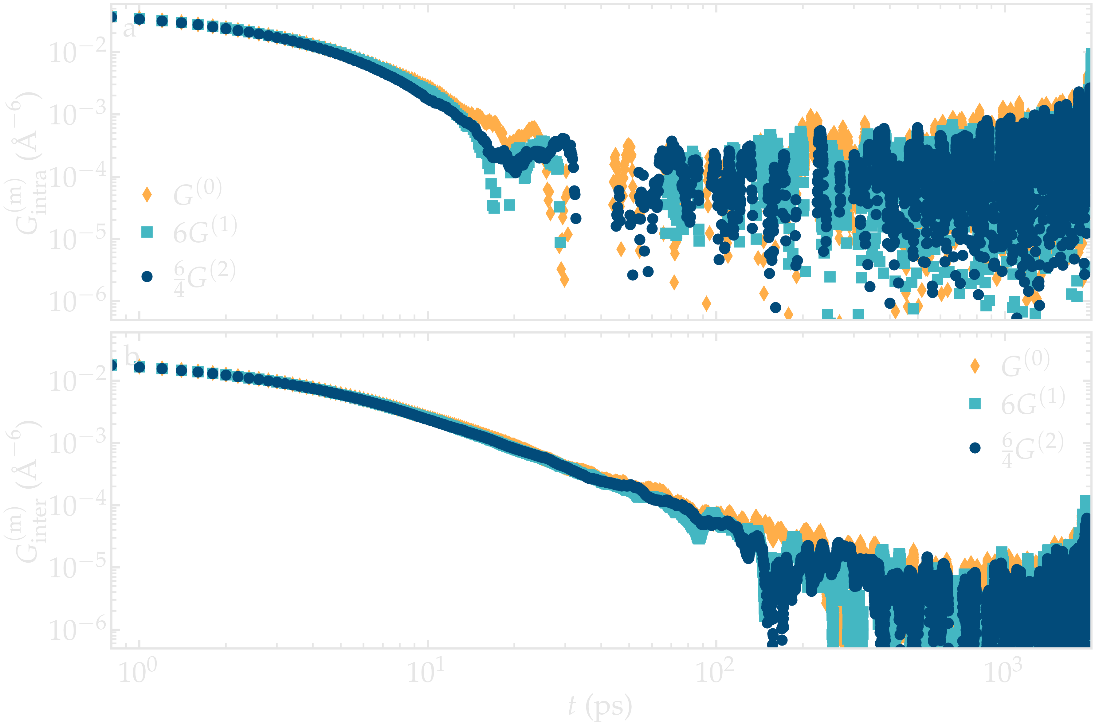
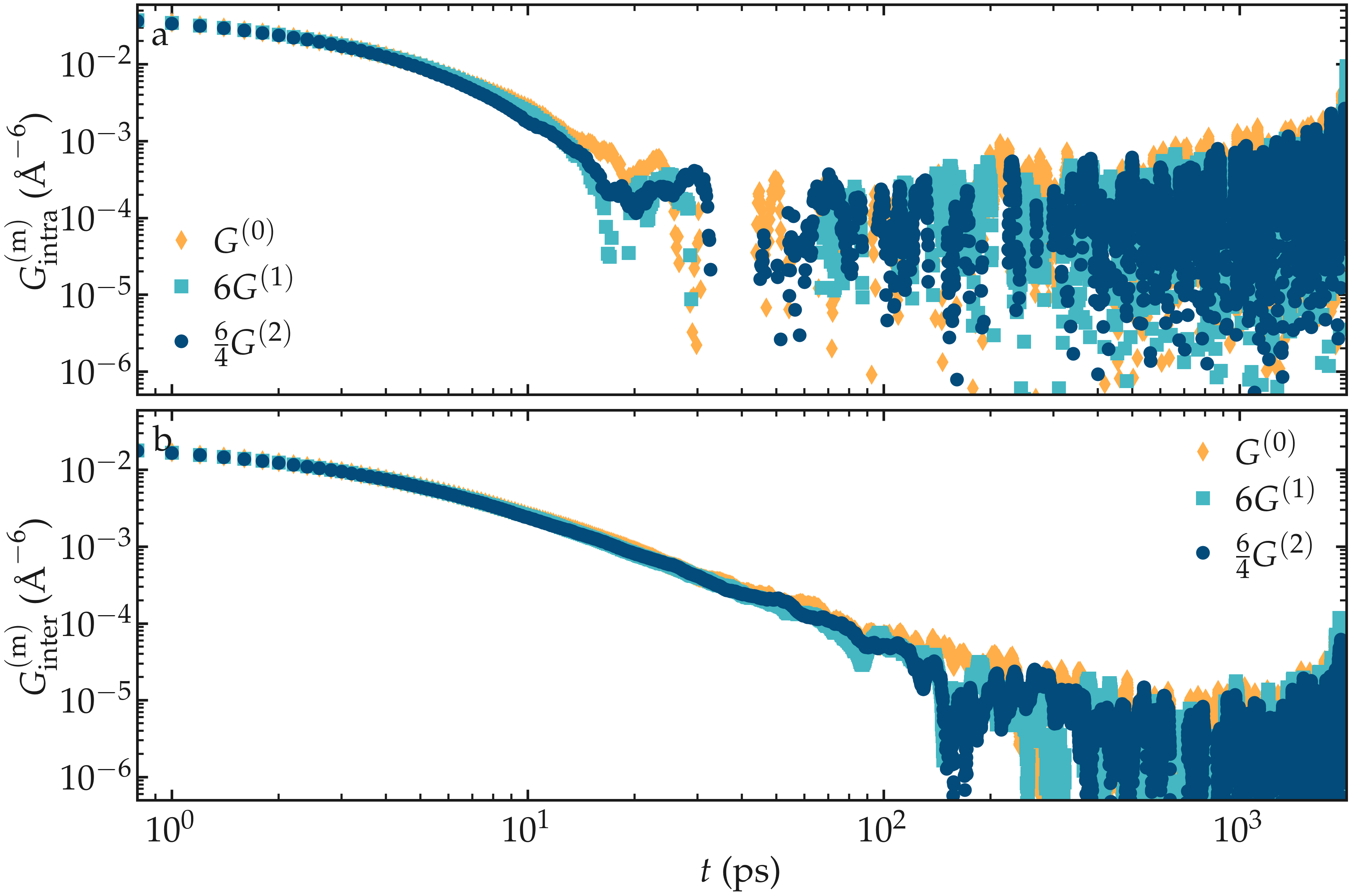
Figure: Validity of the relation \(G^{(0)} = 6 G^{(1)} = 6 / 4 G^{(2)}\) on a bulk water system.