Anisotropic systems

In this tutorial, the NMR relaxation rate \(R_1\) is measured from water confined in a nanoslit os silica.

I recommend you to follow this tutorial on a simpler Isotropic systems first.

MD system

Measuring the NMR relaxation time of nanoconfined water

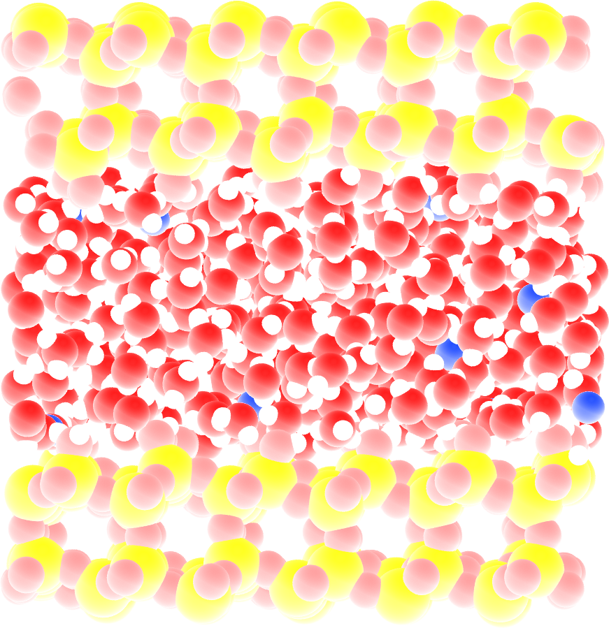
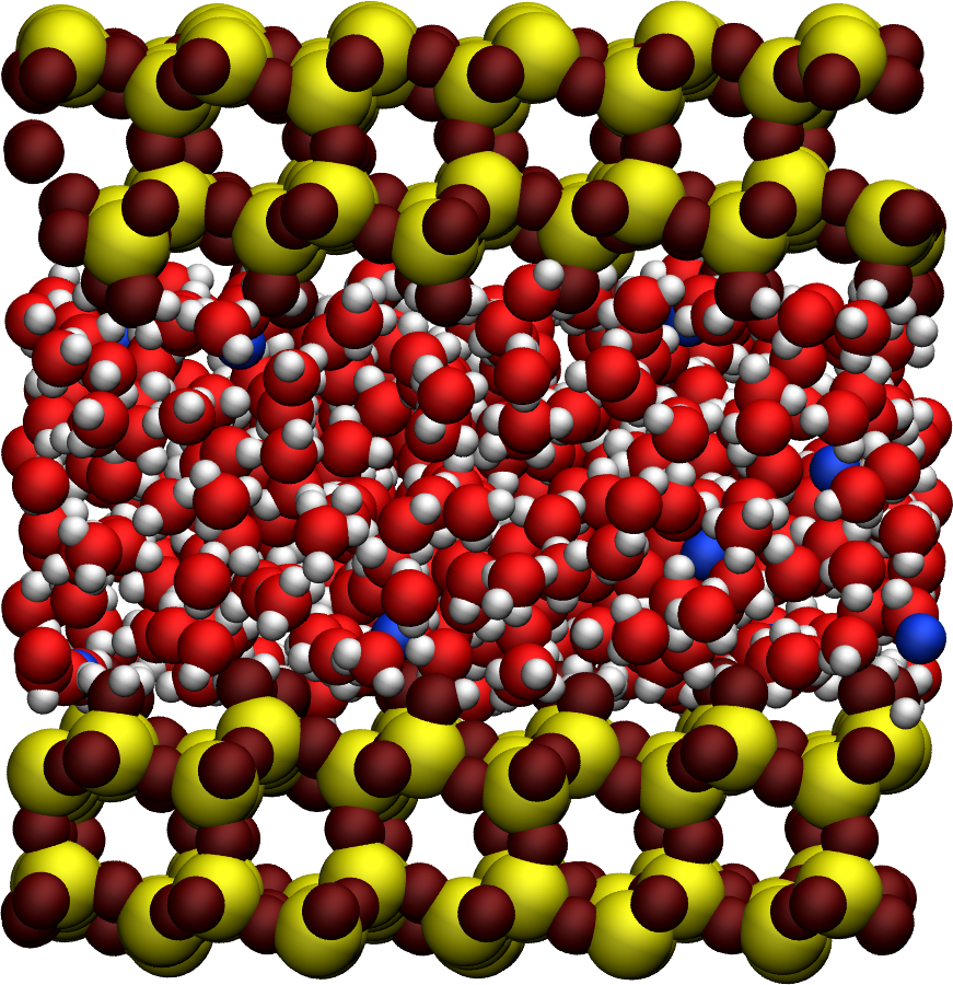
The system is made of 602 \(\text{TIP4P}-\epsilon\) water molecules in a slit silica nanopore. The trajectory was recorded during a \(10\,\text{ns}\) production run performed with the open source code GROMACS in the anisotropic NPzT ensemble using a timestep of \(1\,\text{fs}\). In order to balance the charge of the surface, 20 sodium ions are present in the slit. The imposed was temperature \(T = 300\,\text{K}\), and the pressure \(p = 1\,\text{bar}\). The positions of the atoms were recorded in the prod.xtc file every \(2\,\text{ps}\).

If you are not familiar with GROMACS, you can find tutorials here.

File preparation

To access all trajectory and input files, download the water-in-silica repository from Github, or simply clone it on your computer using:

git clone https://github.com/simongravelle/water-in-silica.git

The dataset required to follow this tutorial is located in raw-data/N50/.

Create a MDAnalysis universe

Open a new Python script or a new notebook, and define the path to the data files:

datapath = "mypath/water-in-silica/raw-data/N50/"

Then, import numpy, MDAnalysis, and NMRforMD:

import numpy as np
import MDAnalysis as mda
import nmrformd as nmrmd

From the trajectory files, let us create a MDAnalysis universe. Import the configuration file and the trajectory:

u = mda.Universe(datapath+"prod.tpr", datapath+"prod.xtc")

Let us extract a few information from the universe, such as number of molecules, timestep, and total duration:

n_molecules = u.atoms.n_residues
print(f"The number of molecules is {n_molecules}")
timestep = np.int32(u.trajectory.dt)
print(f"The timestep is {timestep} ps")
total_time = np.int32(u.trajectory.totaltime)
print(f"The total simulation time is {total_time} ps")

>> The number of molecules is 623
>> The timestep is 2 ps
>> The total simulation time is 10000 ps

Launch the NMR analysis

Let us create 3 atoms groups for respectively the hydrogen atoms of the silica, the hydrogen atoms of the water, and all the hydrogen atoms:

H_H2O = u.select_atoms("name HW1 HW2")
H_SIL = u.select_atoms("name H")
H_ALL = H_H2O + H_SIL

Then, let us run 3 separate NMR analyses, one for the water-silica interaction only, one for the intra-molecular interaction of water, and one for the inter-molecular inter-molecular interaction of water:

nmr_H2O_SIL = nmrmd.NMR(u, atom_group = H_H2O,
                    neighbor_group = H_SIL, number_i=40, isotropic=False)
nmr_H2O_INTRA = nmrmd.NMR(u, atom_group = H_H2O, neighbor_group = H_H2O, number_i=40,
                        type_analysis = 'intra_molecular', isotropic=False)
nmr_H2O_INTER = nmrmd.NMR(u, atom_group = H_H2O, neighbor_group = H_H2O, number_i=40,
                        type_analysis = 'inter_molecular', isotropic=False)

Note the use of isotropic = False, which is necessary here since the system is non-isotropic.

Extract the NMR spectra

Let us access the NMR relaxation rate \(R_1\):

R1_spectrum_H2O_SIL = nmr_H2O_SIL.R1
R1_spectrum_H2O_INTRA = nmr_H2O_INTRA.R1
R1_spectrum_H2O_INTER = nmr_H2O_INTER.R1
f = nmr_H2O_SIL.f

The 3 spectra \(R_1\) can be plotted as a function of \(f\) using pyplot.

from matplotlib import pyplot as plt
plt.loglog(f, R1_spectrum_H2O_SIL, 'o')
plt.loglog(f, R1_spectrum_H2O_INTRA, 's')
plt.loglog(f, R1_spectrum_H2O_INTER, 'd')
plt.show()

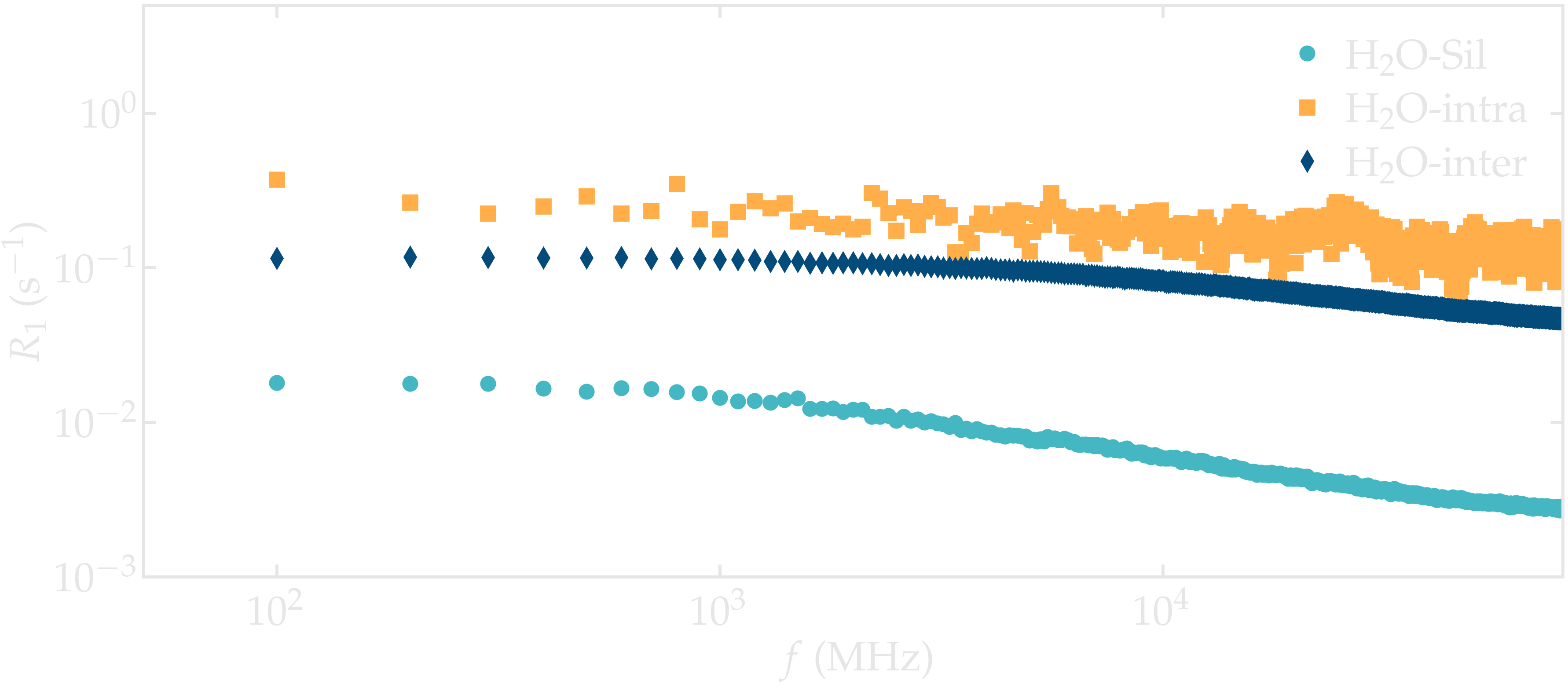
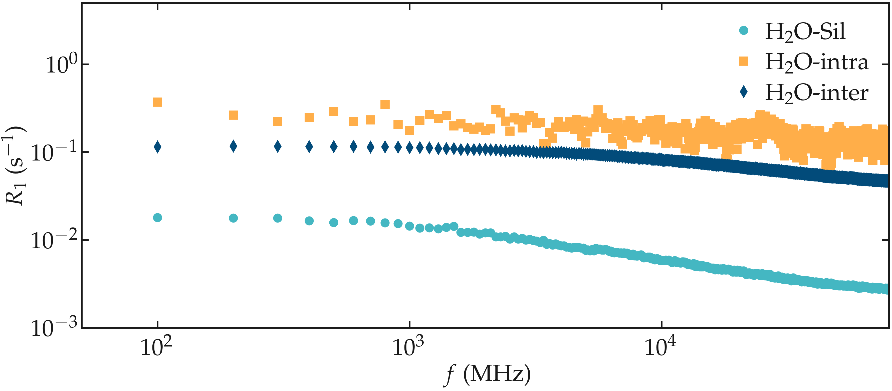
Figure: NMR relaxation rates \(R_1\) for the water confined in a silica slit.

Note that the \(\text{H}_2\text{O}-\text{silica}\) contribution is much smaller than the intra and inter molecular contribution from the water. This can be explained by the comparatively small number of hydrogen atoms from the silica: 92, compared to the 1204 hydrogen atoms from the water.